Summary statistics of neutral population models

This is all assuming a Wright-Fisher population of discrete non-overlapping generations.

Parameters

There are a fixed number of N individuals.
Mutations enter the population at a rate of μ mutations per individual per site per generation.
In a haploid population (usually the case for pathogens), we summarize the population with the parameter θ, which equals 2Nμ. Without temporally resolved data, it’s not possible to separately estimate N and μ; in most population genetic circumstances, we can only estimate θ. With temporally resolved data we can separate θ into N and μ.

Diversity

Genetic diversity is most commonly summarized with the statistic π, which is equal to the average number of mutations per site between two random individuals in the population. π is most commonly measured in terms of substitutions per site. The expectation of π follows

\displaystyle E[\pi] = \theta = 2N\mu

π for Drosophila and π for flu is approximately 0.01, while π for humans is approximately 0.001. This means that for an average length gene of 1000 basepairs, two random fruit flies or two random flues will probably differ at ~10 sites, while two random humans will differ at ~1 site.

Unique variants

The number of unique haplotypes in a sample of n sequences can be estimated from Ewen’s sampling formula. Ewen’s sampling formula gives the probability of observing a₁ copies of haplotype 1, a₂ copies of haplotype 2, etc… in a sample of n sequences. The sole parameter of the sampling formula is θ. Thus θ is sufficient to predict the entire distribution of haplotype frequencies. The expectation of k unique haplotypes follows:

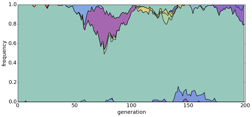
\displaystyle E[k] = \sum^{n}_{i=1} \frac{\theta}{\theta + i - 1}

With θ = 0.2, there is usually only a single dominant haplotype in the population.

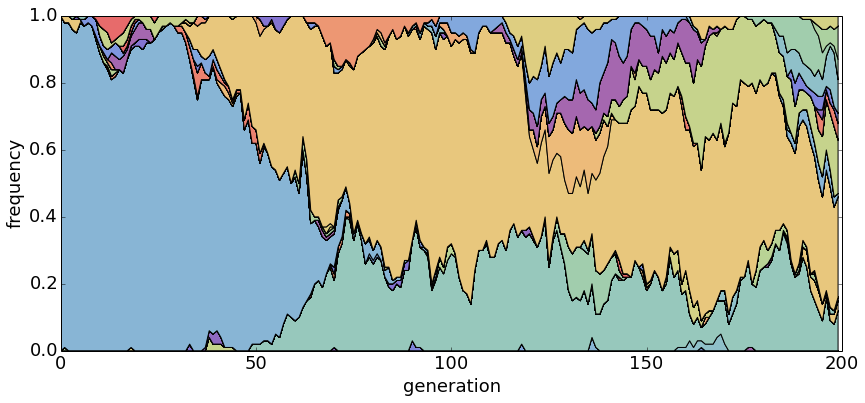
With θ = 1.0, there are generally a small handful of haplotypes.

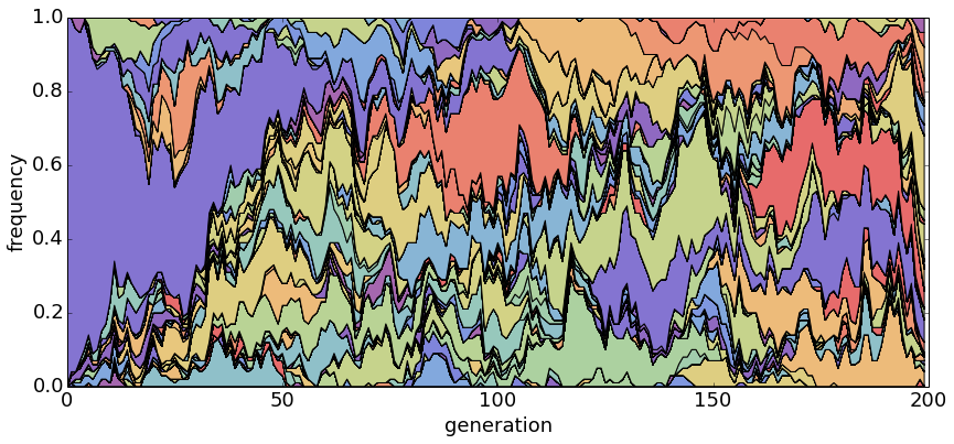
With θ = 5.0, there are many segregating haplotypes.

Chance of fixation

A new mutant appears in the population at an initial frequency p of $1/N$ . It has a $1/N$ of eventually fixing in the population and a $(N-1)/N$ chance of being lost from the population.

Similarly, if a mutant is at population frequency p, then it has a p chance of fixing. At any point in time, looking forwards, the chance of fixation of a neutral mutation is just its frequency.

Time to fixation

Conditioned on a neutral mutant fixing, the expected time to fixation is 2N generations. Thus, the rate of population turnover scales inversely with population size. This time to fixation is also a measure of the strength of random genetic drift.

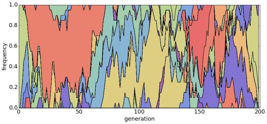
With θ = 1 and N = 20, haplotypes emerge and disappear rapidly.

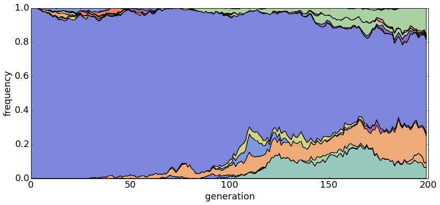
With θ = 1 and N = 100, population turnover takes approximately 200 generations.

With θ = 1 and N = 500, population turnover occurs slowly.

Divergence

Each generation we expect Nμ mutations across the entire population. Each mutation has a $1/N$ chance of fixing. Thus the rate of fixed mutations is $N \mu \times 1/N = \mu$ .

This result, that the rate of neutral divergence across a species is equal to the rate of mutation in a single individual, is a classic finding from Kimura.

Overview

Mutation rate μ determines the rate of interspecies divergence, population size N determines the rate of population turnover and their product Nμ determines the level of standing genetic variation.