Molecular clocks and the coalescent
Trevor Bedford (@trvrb)
May 26, 2020
GS541 Introduction to Computational Molecular Biology
Molecular clocks and dated phylogenies
Mutations tend to accumulate in a clock-like fashion
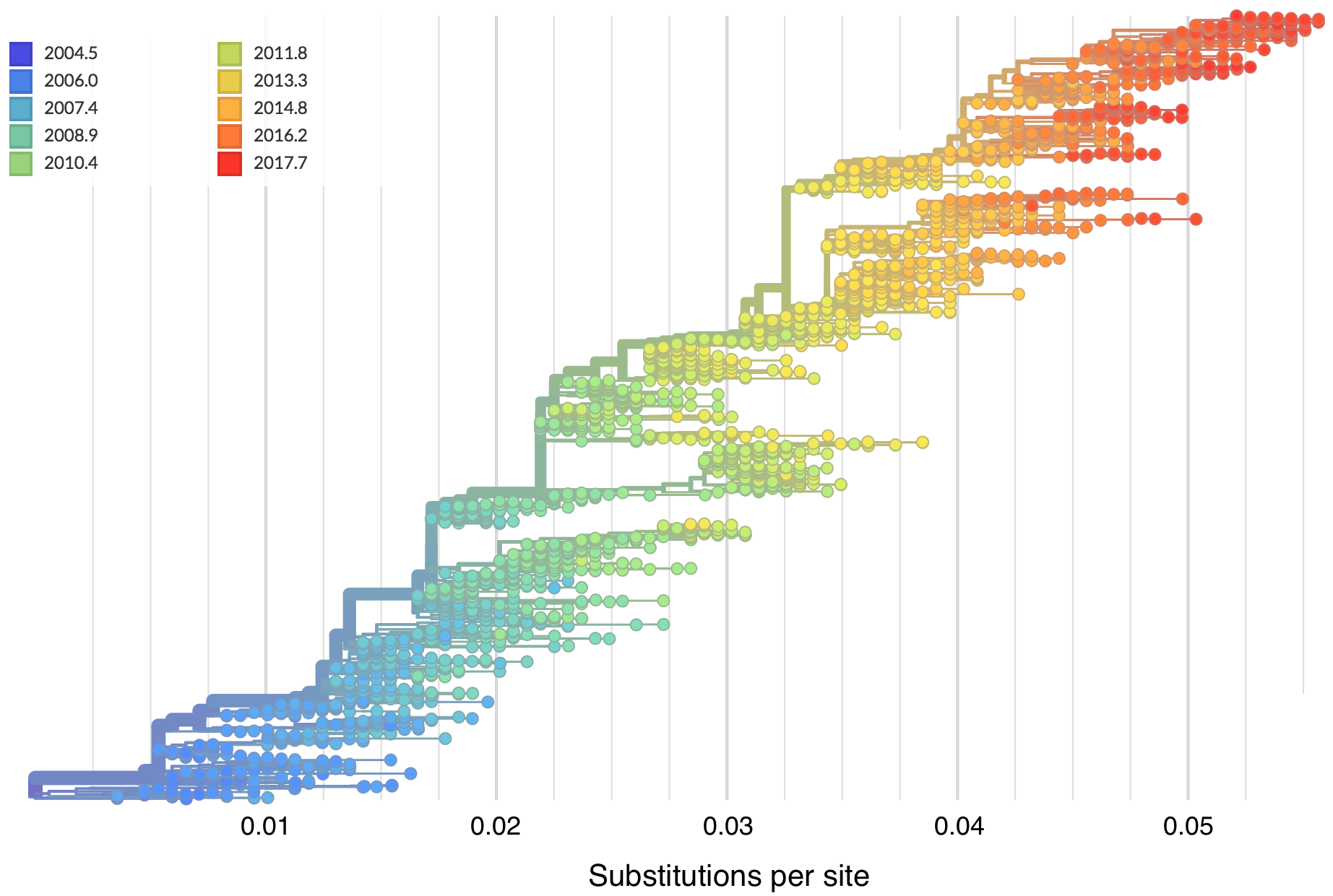
"Root-to-tip" plots show temporal signal
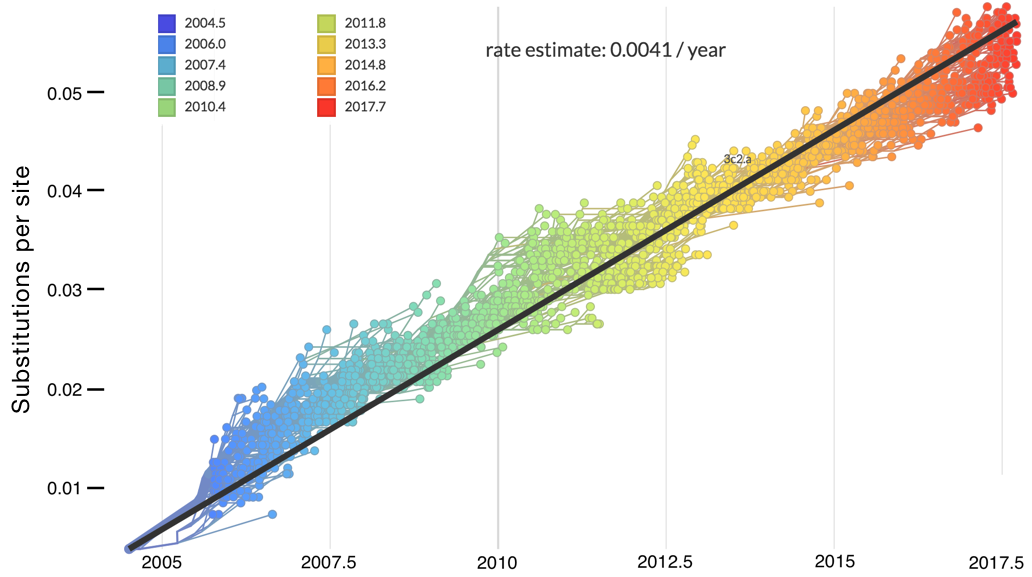
Allows conversion between branch length and time
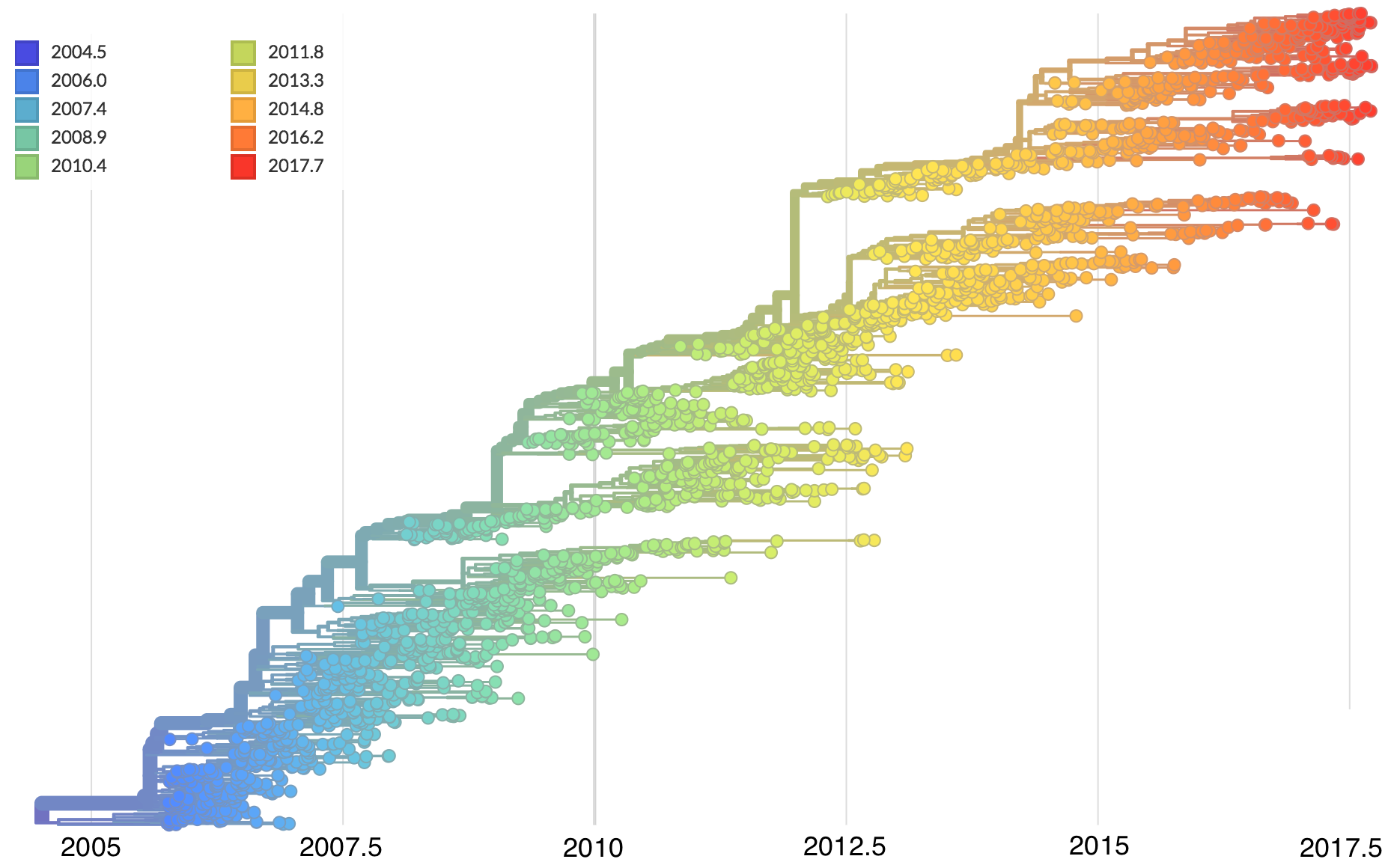
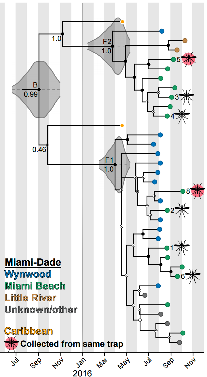
Dated phylogenies provide real-world context
Conversion between mutations and time

Taxa A and B are separated by 1 mutation, where divergence is low relative to alignment length, ie 1 mutation in a 30 kb genome. Evolutionary rate μ = 2 mutations per month.
This is a Poisson process in which k events are observed in an unknown amount of time t, but with known rate μ. $k \sim Poisson(\mu \, t)$
Conversion between mutations and time

With $k = 1$ and $\mu = 2$, we have $\mathrm{Pr}(k|t) = 2 \, t \, e^{-2 \, t}$
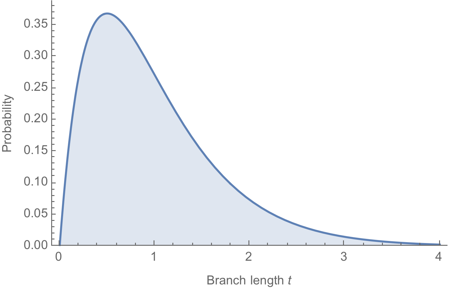
Conversion between mutations and time
Likelihoods multiplied across branches and μ estimated
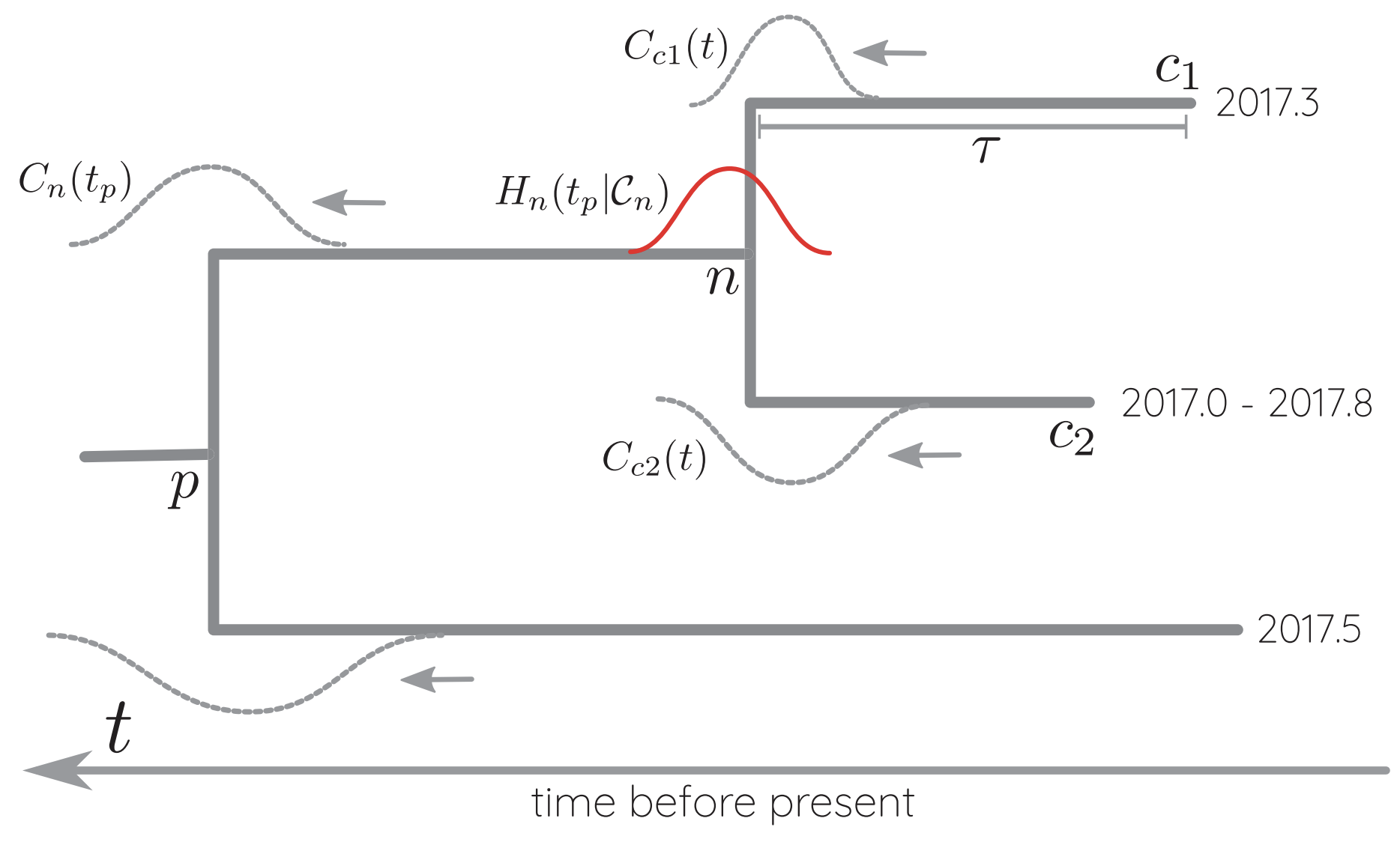
Conversion between mutations and time
Approaches:
- Simple regression of time vs divergence (eg root-to-tip plot)
- Maximum likelihood inference (eg TreeTime)
- Bayesian inference (eg BEAST)
The coalescent
Wright-Fisher process
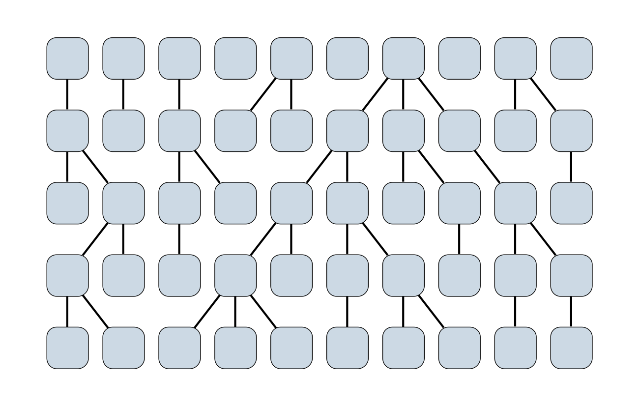
Sample some individuals
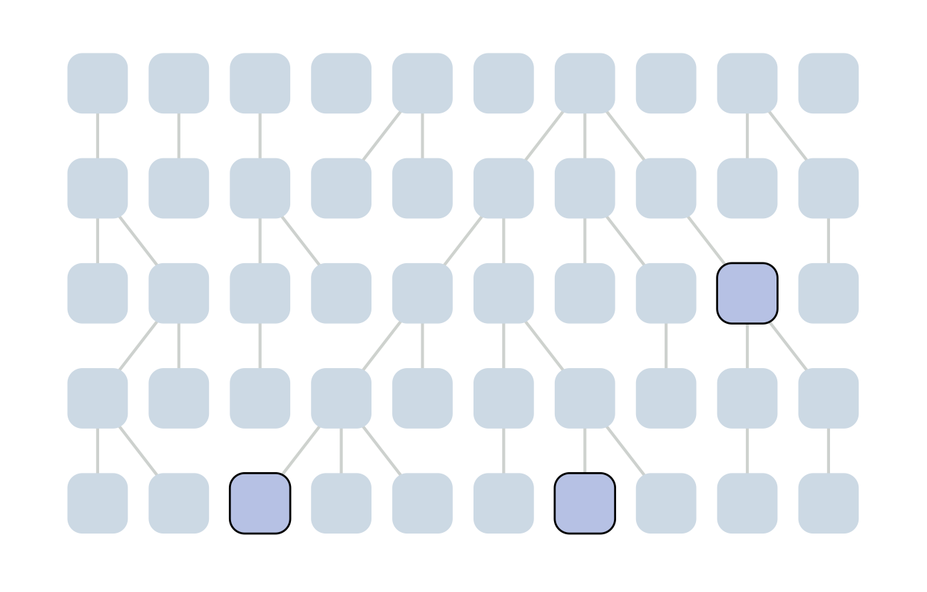
Each generation coalescence may occur
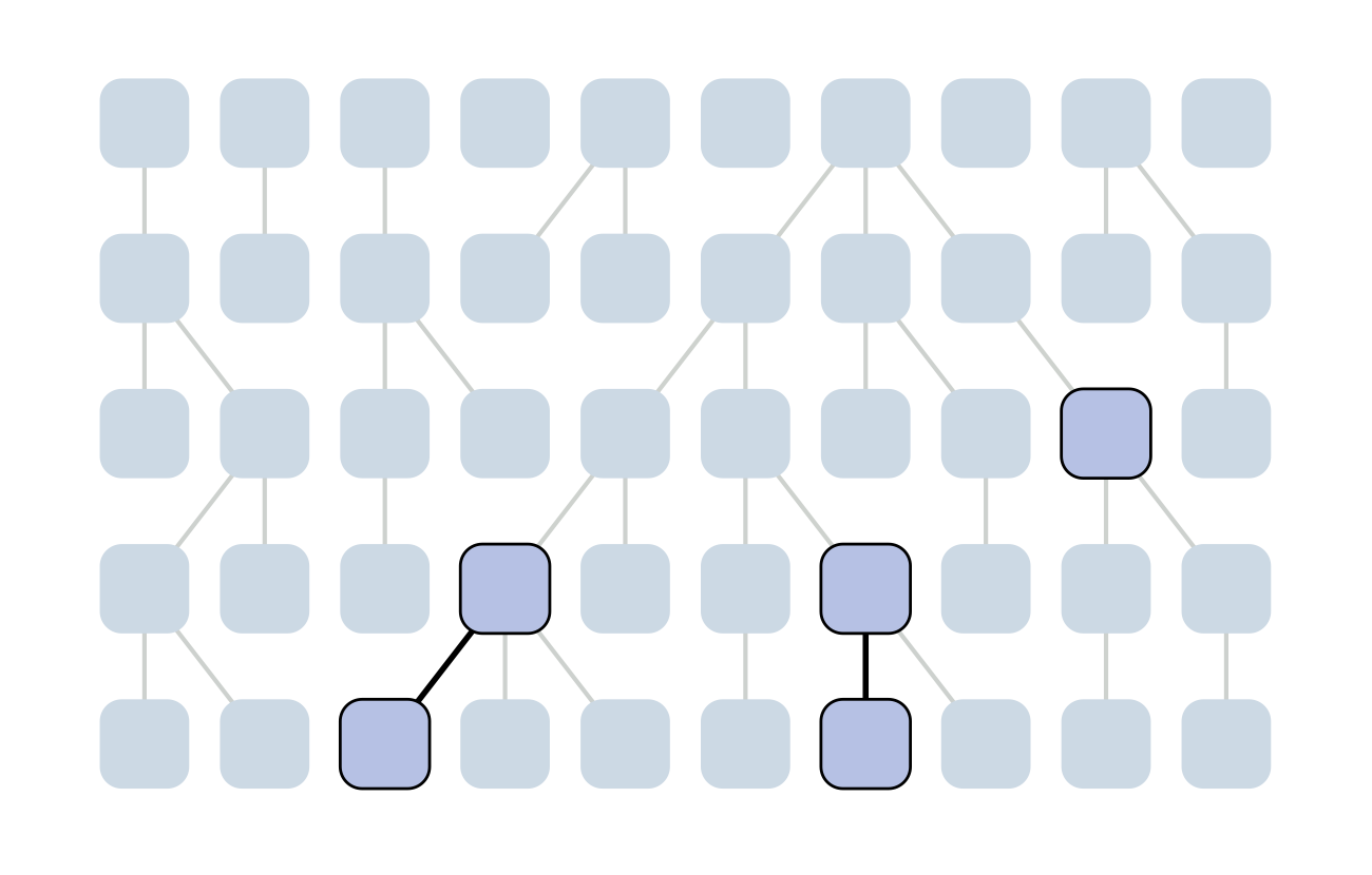
Each generation coalescence may occur
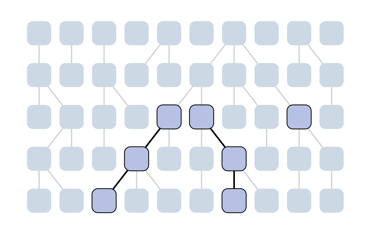
Each generation coalescence may occur
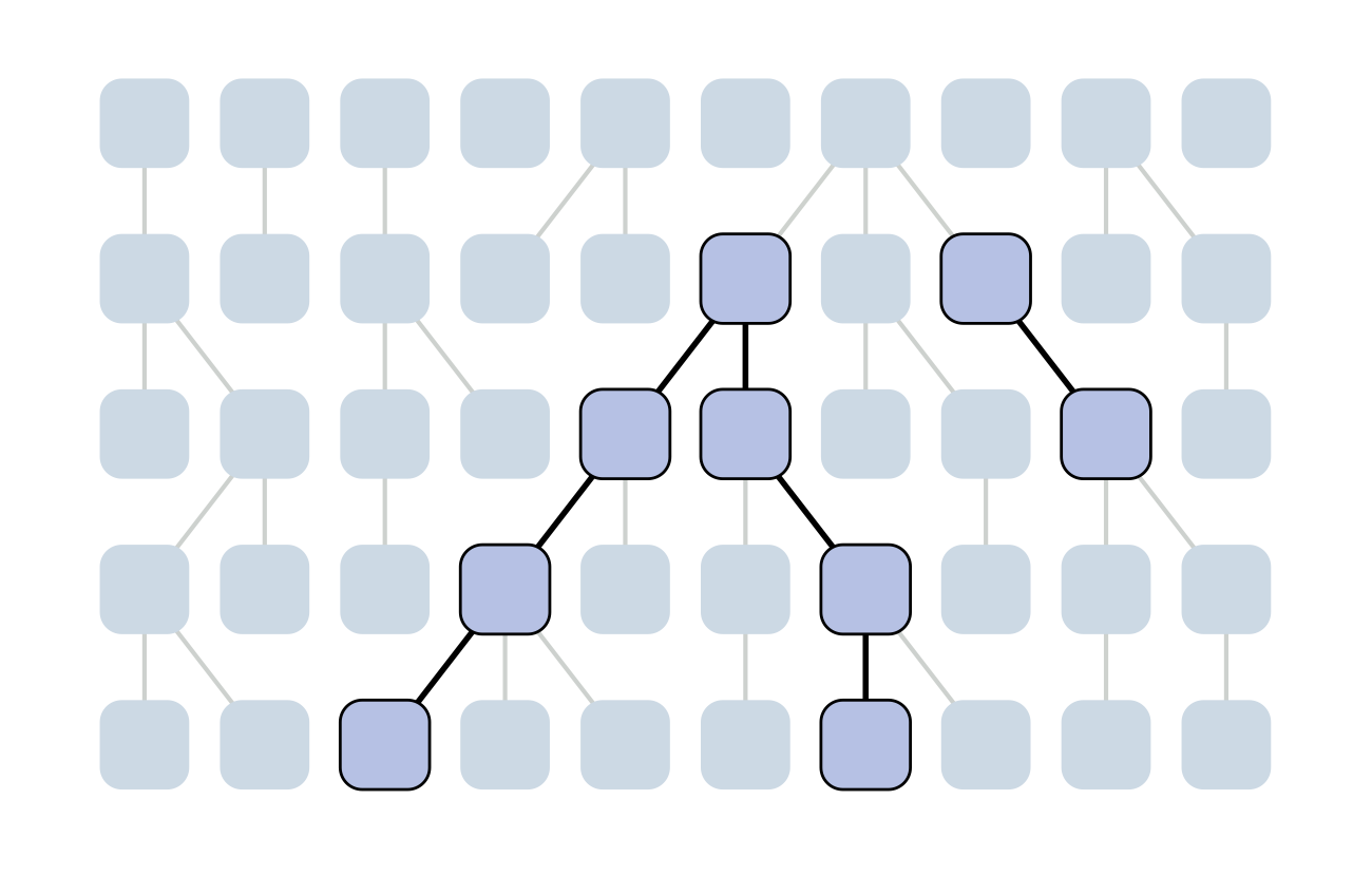
Each generation coalescence may occur
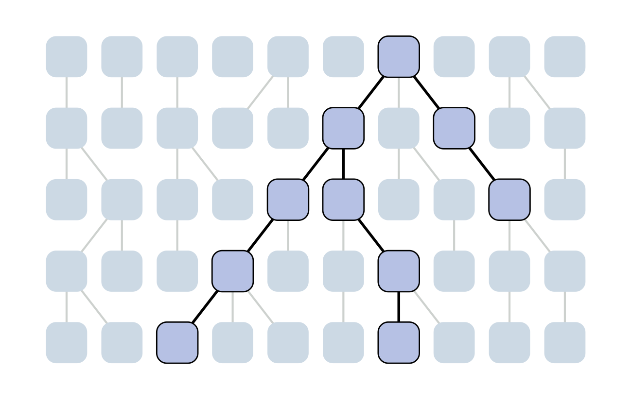

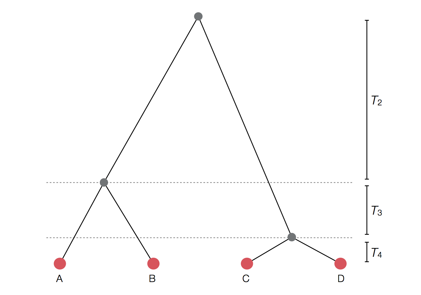
Set of coalescent intervals
Per-generation probability of coalescence
$$\mathrm{Pr}(\mathrm{coal} \, | \, i=2) = \frac{1}{N}$$
Probability of first lineage picking an arbitrary parent is 1, while the probability of the 2nd lineage picking the same parent is $\frac{1}{N}$.
Probability of coalescence scales inversely with population size.
Per-generation probability of coalescence
$$\mathrm{Pr}(\mathrm{coal}) = \binom{i}{2} \frac{1}{N} = \frac{i(i-1)}{2N}$$
There are $\binom{i}{2}$ ways pairs of lineages can pick the same parent.
Probability of coalescence scales quadratically with lineage count.
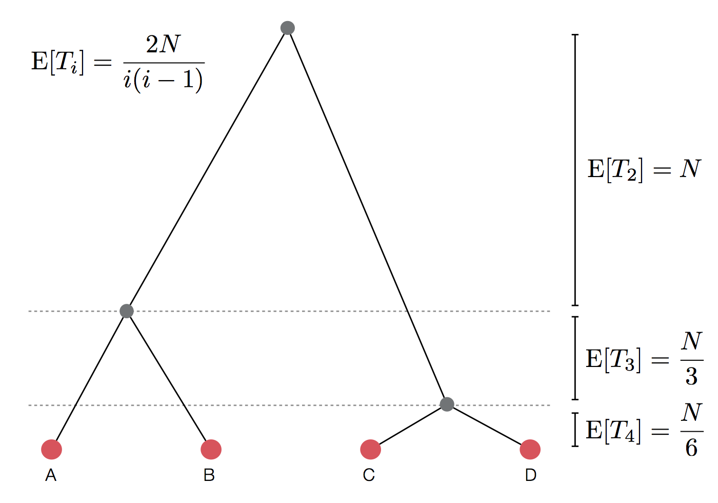
Expected waiting time to coalescence
$$\mathrm{E}[T_i] = \frac{2N}{i(i-1)}$$
This is a geometric distribution. If each generation there is a $\frac{1}{x}$ probability of an event occurring, we expect to wait $x$ generations for the event to occur.
Continuous time limit
With per-generation probability of an event $\frac{1}{x}$ small, but many generations, then the
discrete time geometric distribution approximates to a continuous time
exponential distribution.
Thus, we assume $T_i$ to be exponentially distributed with mean
$$\mathrm{E}[T_i] = \frac{2N}{i(i-1)}.$$
Set of coalescent intervals with waiting times
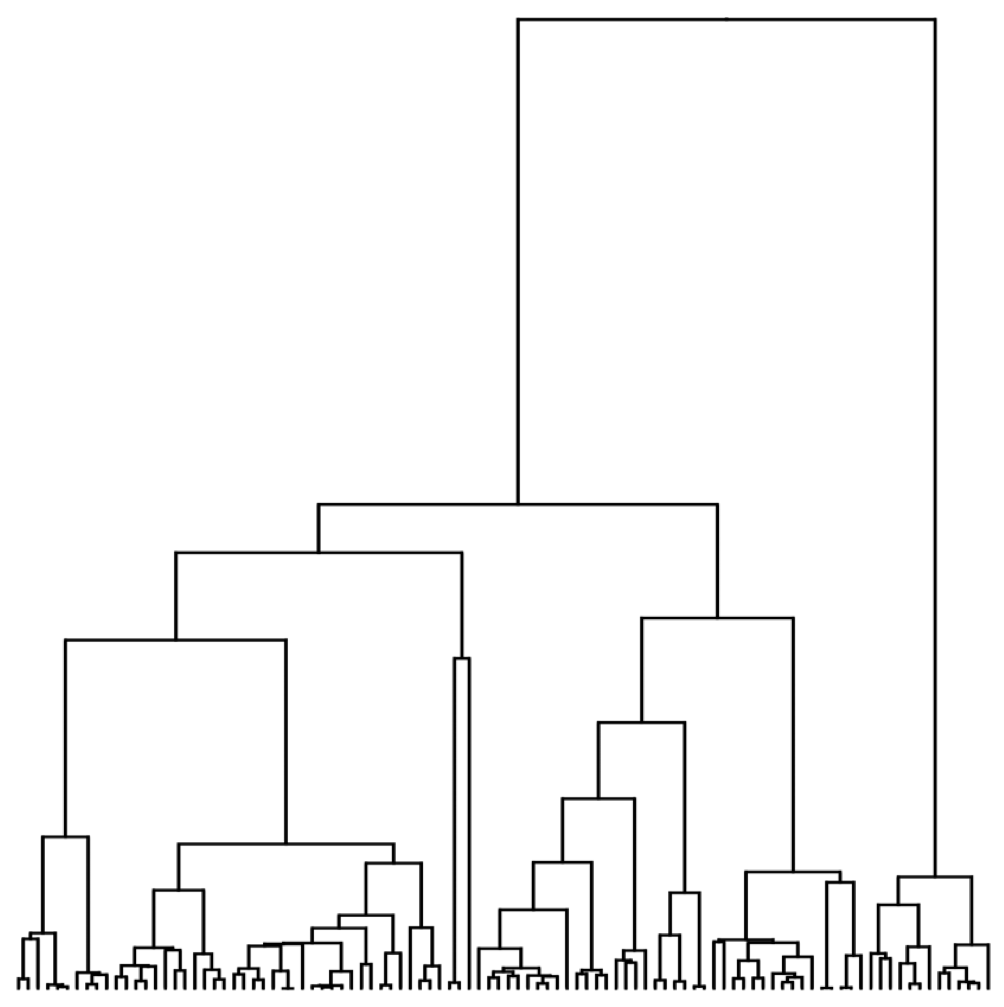
Gives coalescent trees their distinctive shape
Rate of coalescence scales with population size N
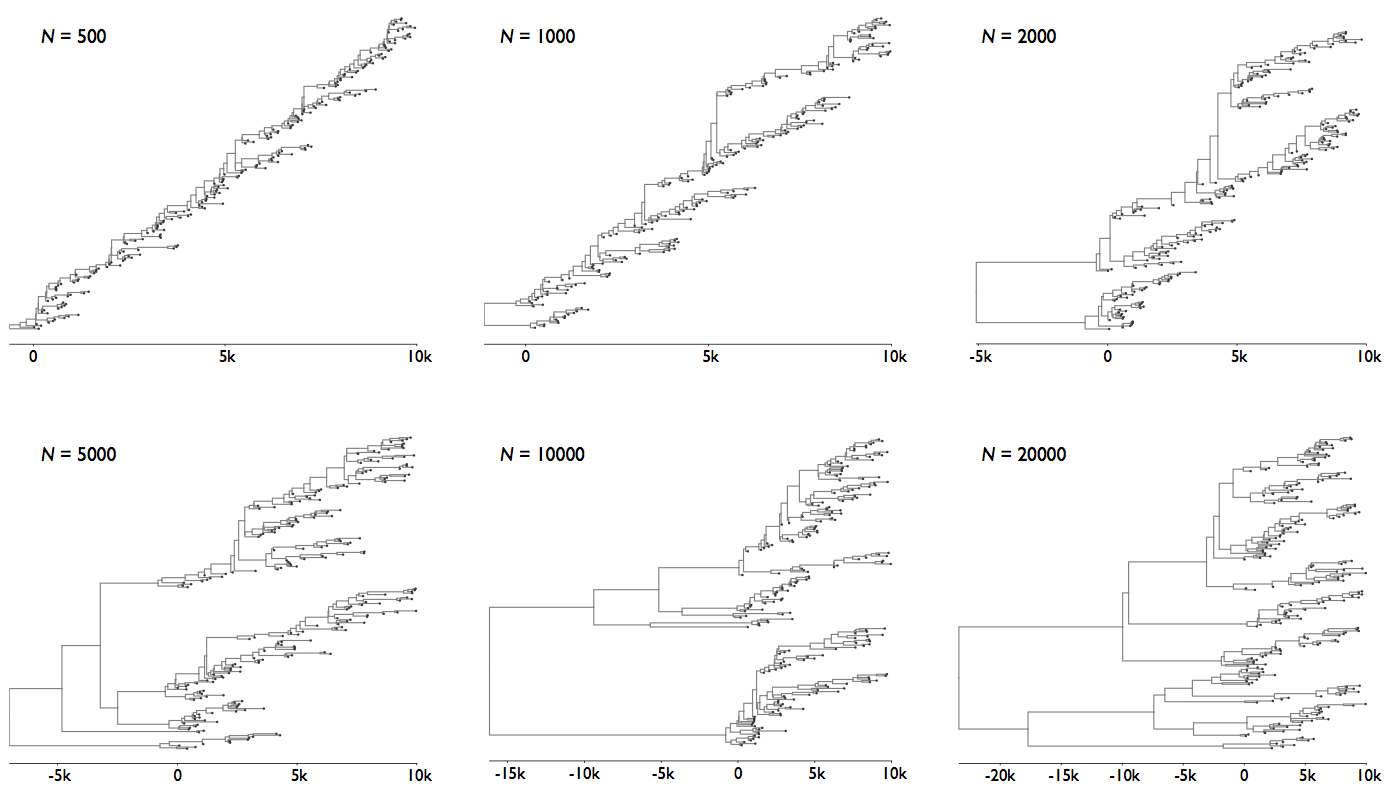
Visualization of the coalescent process
Pairwise genetic diversity
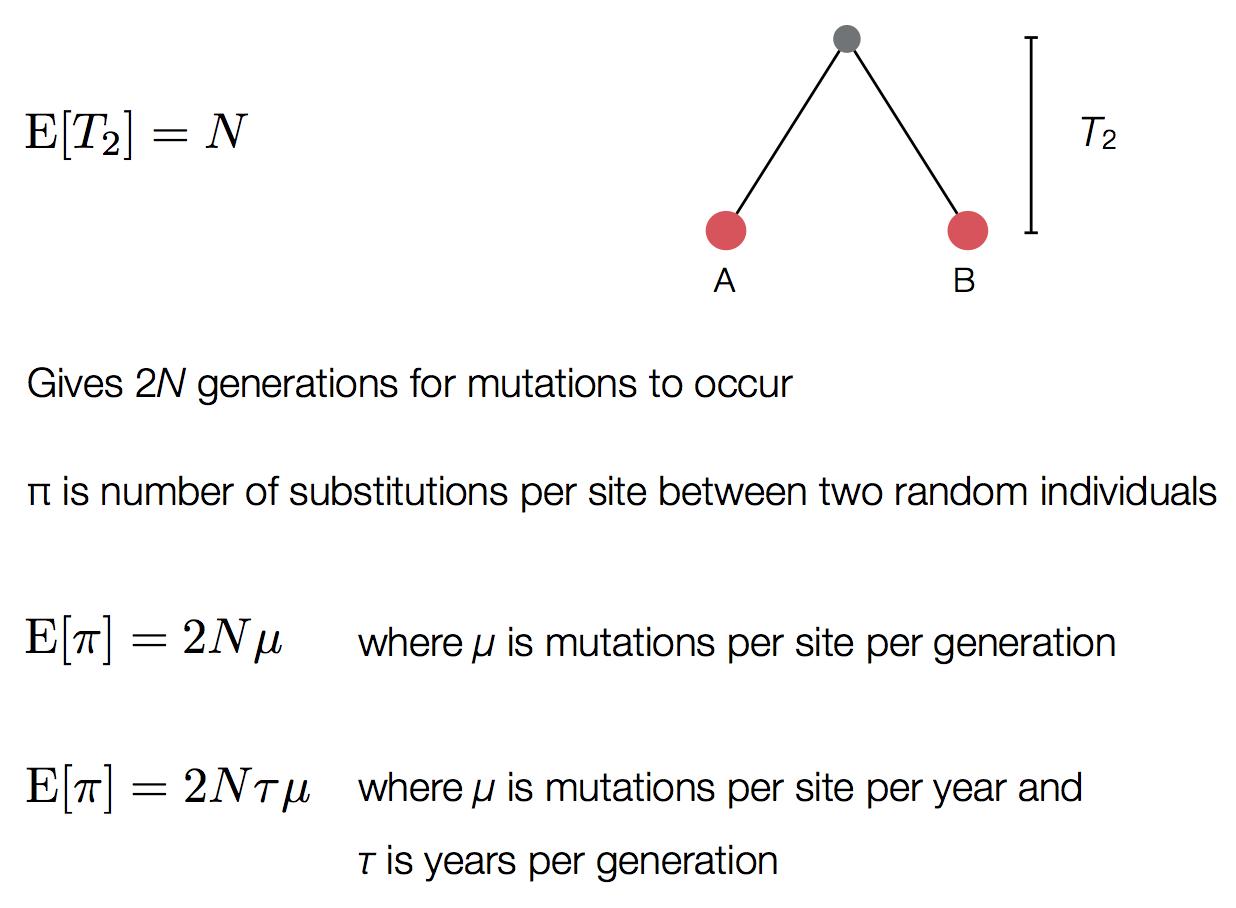
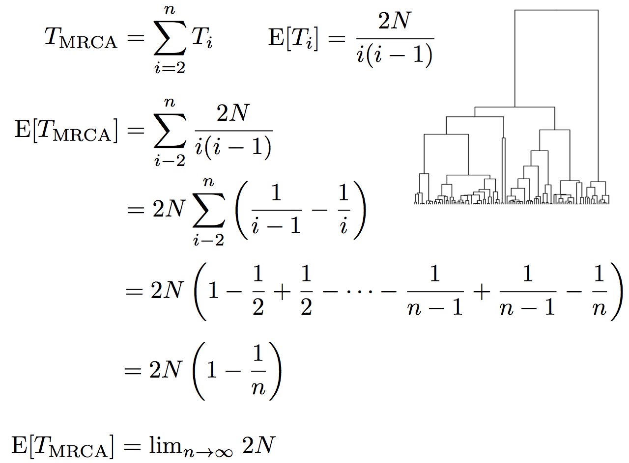
Time to the most recent common ancestor (TMRCA)
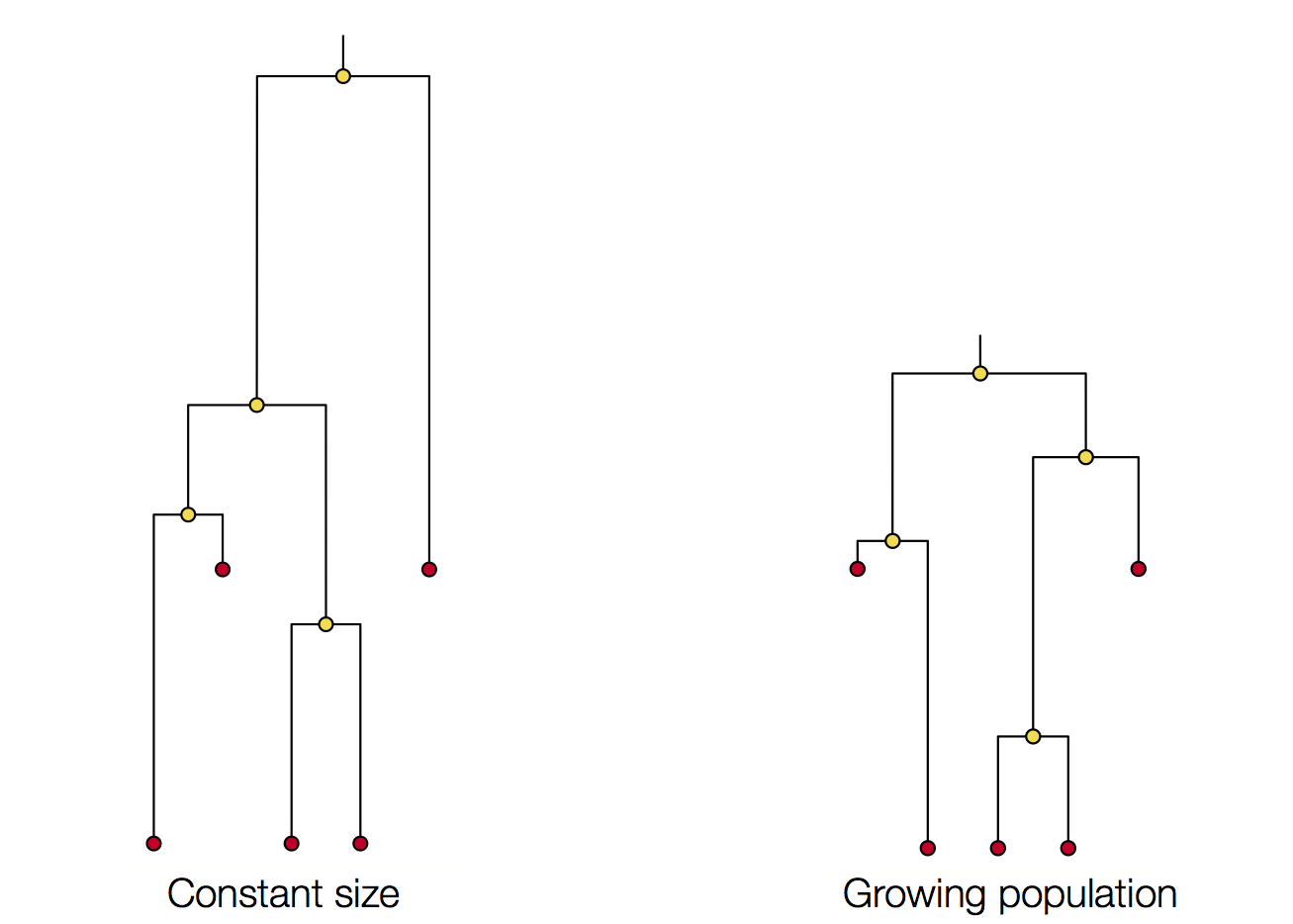
Coalescence patterns can estimate population growth/decline
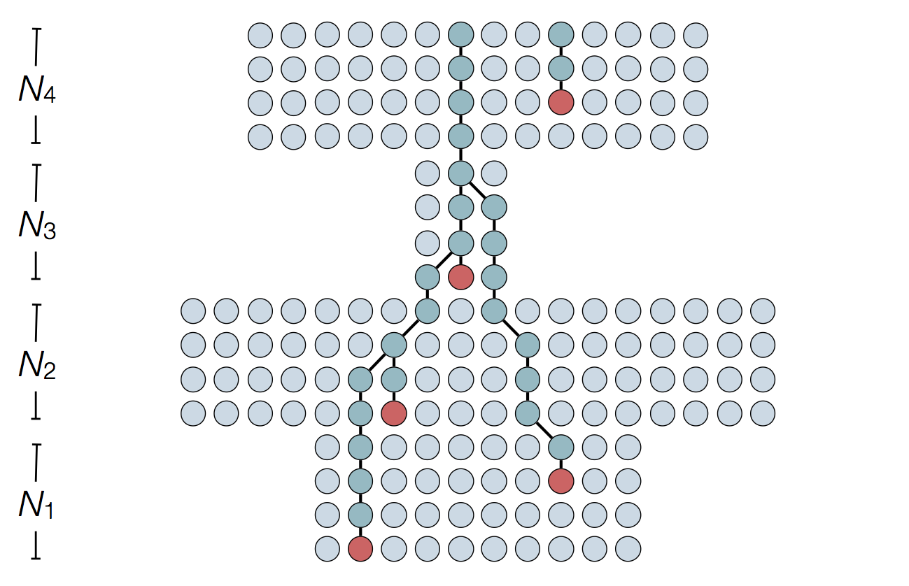
Changing population size alters coalescent rate
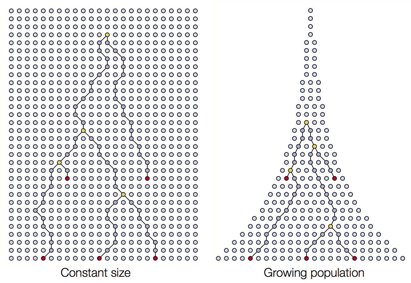
Changing population size alters coalescent rate
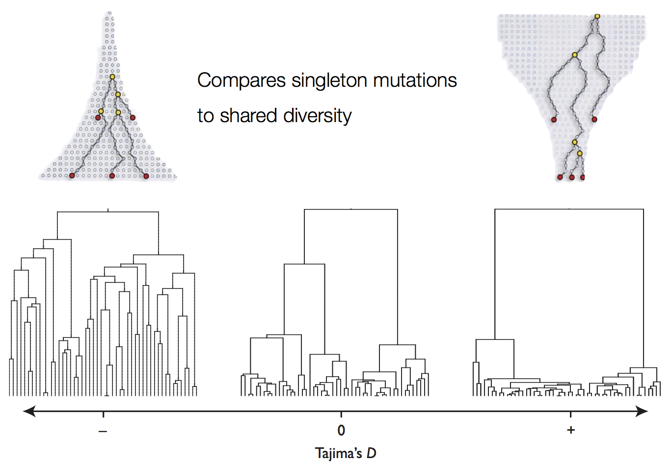
Tajima's D statistic summarizes deviation from neutrality
'Skyline' is flexible demographic model that estimates windows of coalescent rate
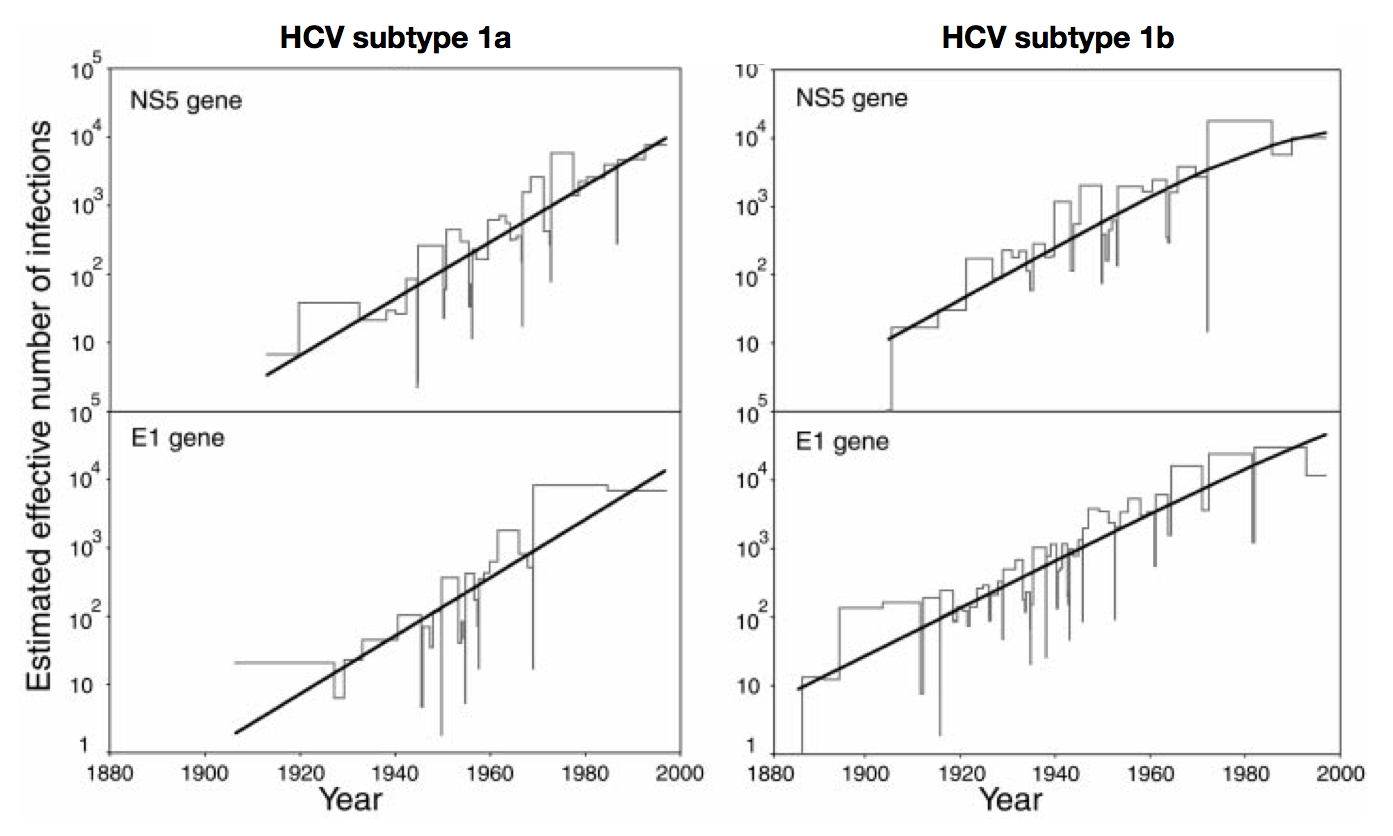
Skyline model shows population growth in HCV
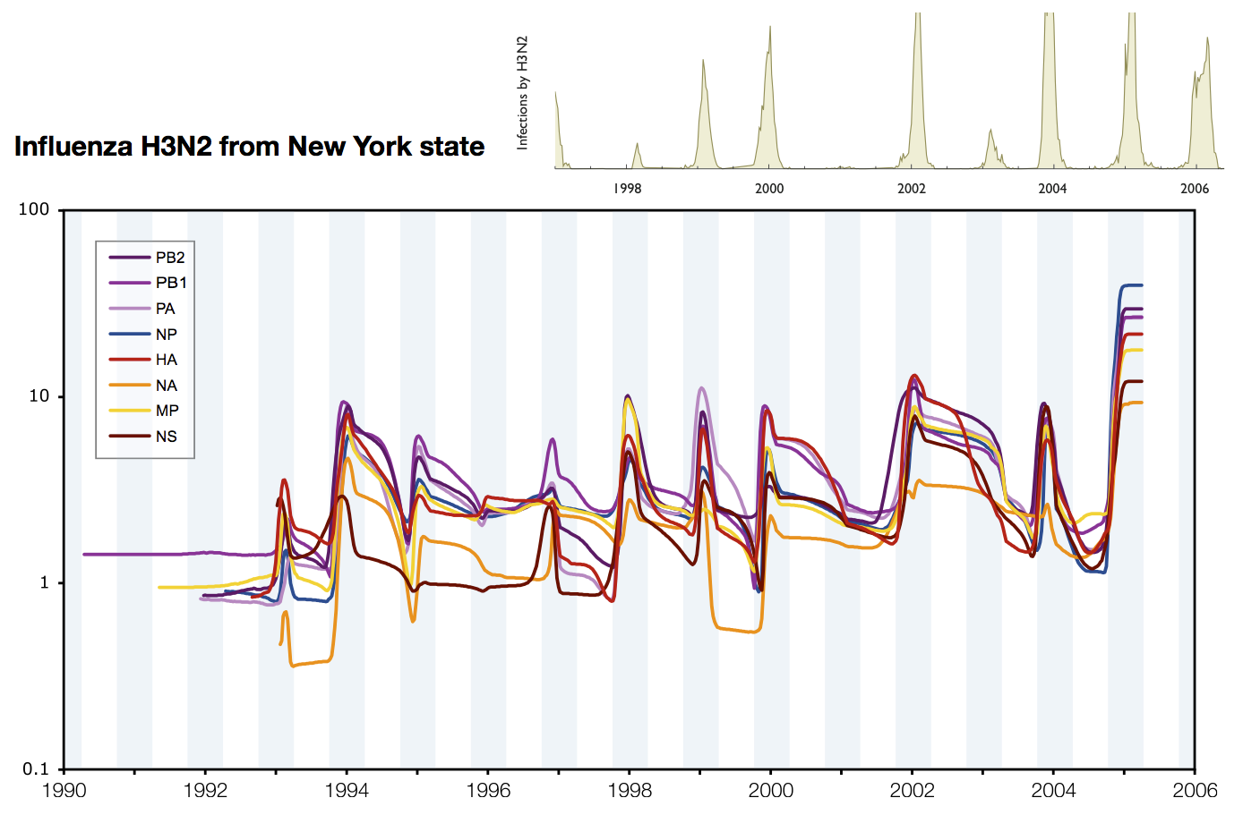
Skyline model shows seasonality in flu
Interpreting rate of coalescence
These approaches directly estimate the pairwise rate of coalescence $\lambda$, which is measured in terms of events per year. Thus, the timescale of coalescence $\frac{1}{\lambda}$ is measured as the expected waiting time in years for two lineages to find a common ancestor.
Interpreting rate of coalescence
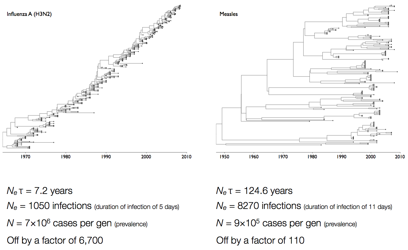
The timescale of coalescence $\frac{1}{\lambda}$ is equal to $N_e\tau$, where $N_e$ is measured in generations and $\tau$ is measured in years per generation. $\tau$ acts to rescale time from generations to years.
Example tree
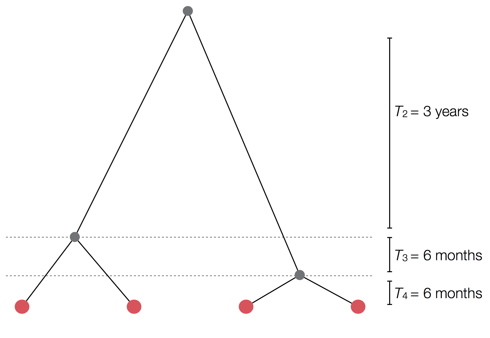
Example skyline plot
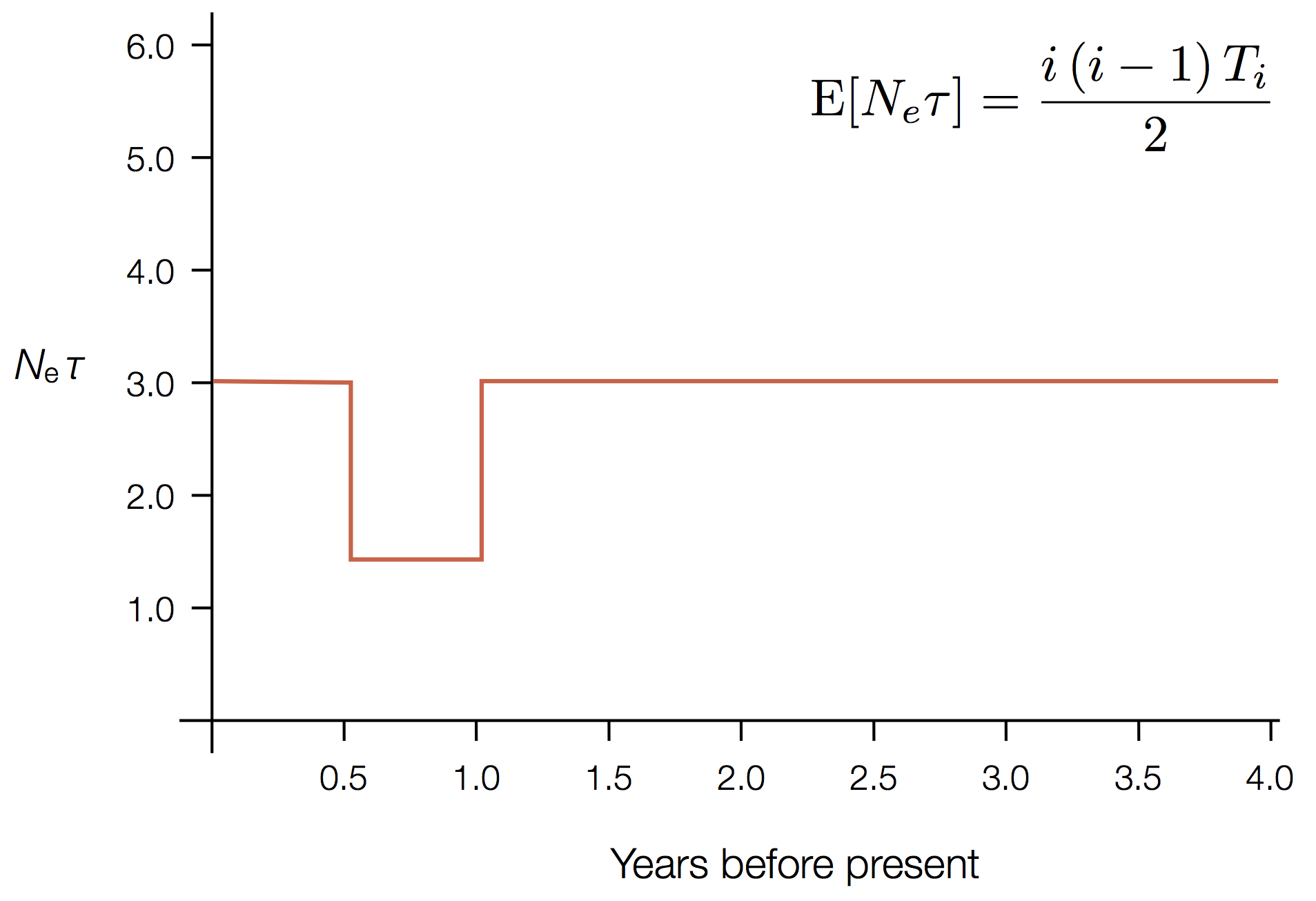
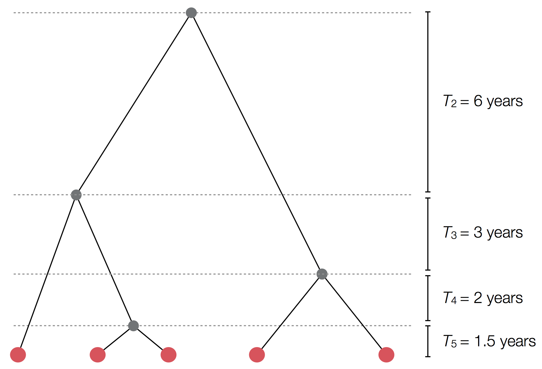
Exercise: plot skyline from tree
Influenza phylogeny and effective number of infections
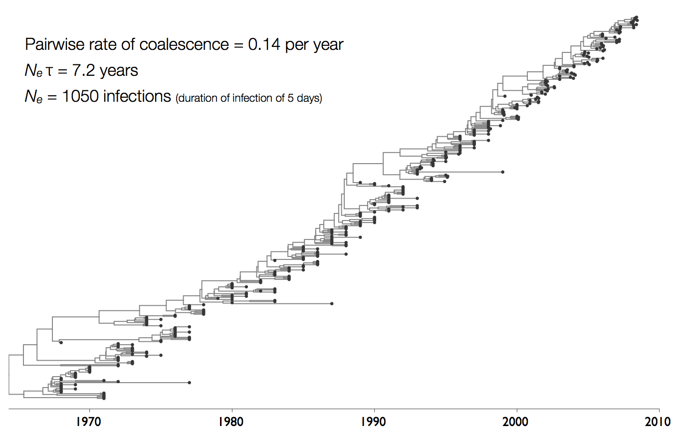
Coalescent rates in flu and measles
Coalescent analyses of SARS-CoV-2